Inventory Control with Ordering Costs
This example studies a 12-period stochastic lot-sizing problem with two formulations — a relaxed (continuous) case and an integer (MIP) case with fixed ordering costs. The comparison shows:
- Relaxed problem: SDDP with a PAR(1) demand approximation is near-optimal and outperforms TS-DDR.
- Integer problem: TS-DDR with
FixedDiscreteIntegerStrategyoutperforms both SDDP and TS-DDR withContinuousRelaxationIntegerStrategy, because SDDP and continuous relaxation both underestimate the fixed ordering cost.
using DecisionRules
using JuMP, HiGHS
using Flux
using Statistics, Random
Information Pattern
At the beginning of a period, the controller observes current inventory and recent realized demand. It does not observe current demand before ordering. The order is therefore ex-ante. After ordering, demand is realized and becomes part of the state for the next period.
The state carried between periods is:
[net_inventory, last_demand, previous_demand]This lets a time-invariant policy infer the latent demand regime from recent observations without receiving a period counter or synthetic seasonal features.
Inventory Model
Relaxed formulation
The order quantity is continuous with no setup cost:
\[0 \le q_t \le Q_{\max}, \qquad \text{cost}_t = c\,q_t + h\max(s_t,0) + p\max(-s_t,0).\]
Integer formulation
A binary variable $z_t \in \{0,1\}$ controls whether an order is placed. If $z_t = 0$, then $q_t$ must be zero; if $z_t = 1$, the model pays a fixed setup cost $K$:
\[0 \le q_t \le Q_{\max}\,z_t, \qquad \text{cost}_t = K\,z_t + c\,q_t + h\max(s_t,0) + p\max(-s_t,0).\]
In both cases, ordered units arrive before demand:
\[s^{mid}_t = s_{t-1} + q_t, \qquad s_t = s^{mid}_t - d_t.\]
| Parameter | Value | Meaning |
|---|---|---|
| $T$ | 12 | periods |
| $K$ | 500 | fixed order/setup cost (integer case) |
| $c$ | 2 | unit ordering cost |
| $h$ | 1 | holding cost |
| $p$ | 25 | backlog penalty |
| $Q_{\max}$ | 350 | order capacity |
| $s_0$ | 30 | initial inventory |
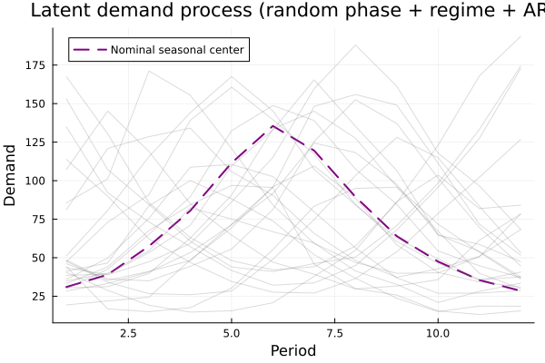
Demand Process
Each trajectory has a path-level phase shift $\phi \sim \mathrm{Unif}\{0,\ldots,T-1\}$, a persistent latent regime $r_t \in \{-1,0,1\}$ (switch probability 0.04), and an autoregressive shock $\epsilon_t$:
\[\epsilon_t = 0.92\,\epsilon_{t-1} + 0.35\,\eta_t, \qquad d_t = \operatorname{clip}\!\bigl( m_{\kappa_t} + w_{\kappa_t}(0.85\,r_t + 0.42\,\epsilon_t + 0.12\,\eta'_t) \bigr),\]
where $\kappa_t = 1 + ((t + \phi - 1) \bmod T)$ is the shifted seasonal index, and $m_{\kappa_t}$ and $w_{\kappa_t}$ are the midpoint and half-width of the seasonal demand band. None of the latent variables are observed; the policy sees only inventory and realized demand history.
The plot below shows 24 sampled demand paths. Because each trajectory has a different phase and persistent regime, the same calendar period can correspond to high, medium, or low demand across scenarios.
Integer Postprocessing Strategies
DecisionRules.jl provides two strategies for extracting gradient information from subproblems with discrete variables:
FixedDiscreteIntegerStrategy: (1) solve the MIP for incumbent binary values $z^*_t$; (2) fix $z_t = z^*_t$ and relax integrality; (3) re-solve the resulting LP; (4) read LP duals as gradient signal. This is the same principle as SDDP.jl's FixedDiscreteDuality.
ContinuousRelaxationIntegerStrategy: relax all binary/integer constraints to continuous bounds (binary → [0,1]), solve the resulting LP, and read duals directly. This is faster (one LP instead of MIP + LP) and gives smoother gradients, but the solution may have fractional integer variables — the gradient does not correspond to any feasible integer assignment.
For the relaxed formulation (no integer variables), NoIntegerStrategy is used and subproblems are solved as-is.
Relaxed (Continuous) Problem
When there are no integer variables, SDDP can model the demand process exactly via a PAR(1) approximation that carries $d_{t-1}$ as a state variable. This makes SDDP near-optimal for the relaxed problem.
SDDP uses a PAR(1) fit: $d_t \approx \mu_t + \alpha(d_{t-1} - \mu_{t-1}) + \omega_t$ with per-stage means $\mu_t$, autocorrelation $\alpha \approx 0.86$, and 9 equiprobable innovation points fitted from 10,000 simulated demand paths.
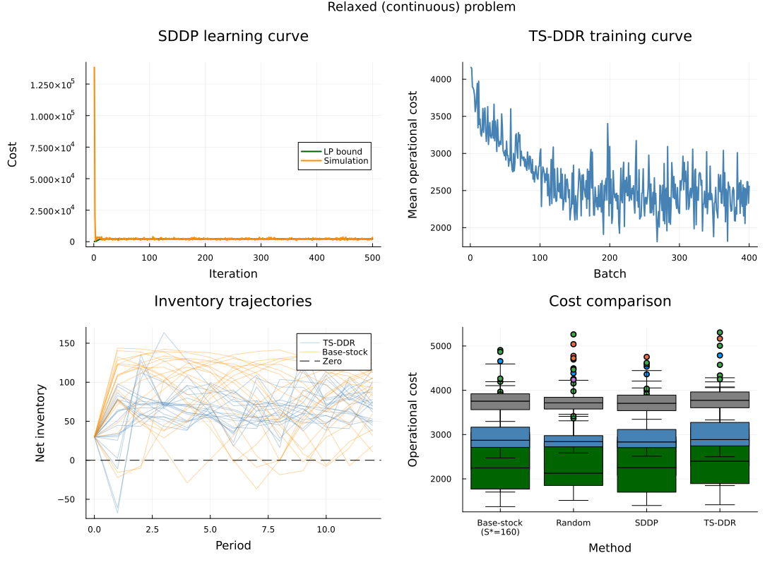
| Method | N | Mean cost | Std | 95% CI | vs TS-DDR | Fit (s) | Eval (s) |
|---|---|---|---|---|---|---|---|
| TS-DDR (trained) | 300 | 2667.3 | 594.5 | 67.3 | +0.0% | 54.6 | 0.0018 |
| SDDP (PAR) | 300 | 2434.2 | 774.8 | 87.7 | -8.7% | 0.0 | 20.6455 |
| Base-stock (S*=160) | 300 | 3035.6 | 506.8 | 57.3 | +13.8% | 0.0 | 0.0002 |
| Random (untrained) | 300 | 3751.7 | 221.7 | 25.1 | +40.7% | 0.0 | 0.0018 |
SDDP clearly dominates: 8.7% lower cost than TS-DDR, 40.7% lower than Random. The SDDP and Random cost distributions are non-overlapping, confirming that informed methods have a clear edge on this demand process.
Integer (MIP) Problem
Introducing the binary $z_t$ and fixed cost $K=500$ changes the landscape. SDDP can only use LP relaxation for training ($z \in [0,1]$), which systematically underestimates $K$: when the LP says $z=0.3$, $q=20$, the relaxed cost is $0.3 \times 500 + 2 \times 20 = 190$, but the true integer cost with $z=1$ is $500 + 40 = 540$.
TS-DDR with FixedDiscreteIntegerStrategy handles this correctly: it solves the full MIP, fixes the binary incumbent, and reads LP duals in that integer-consistent state.
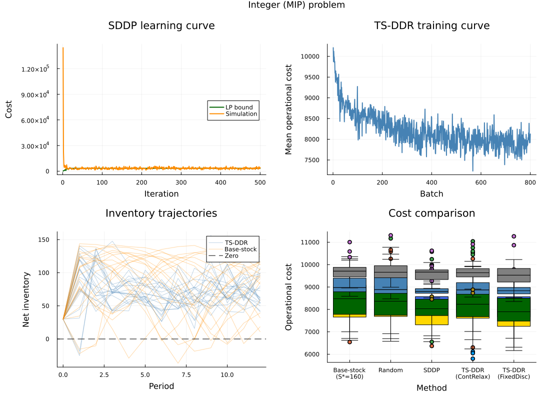
| Method | N | Mean cost | Std | 95% CI | vs TS-DDR (FD) | Fit (s) | Eval (s) |
|---|---|---|---|---|---|---|---|
| TS-DDR (FixedDiscrete) | 300 | 8015.8 | 719.5 | 81.4 | +0.0% | 339.2 | 0.0112 |
| TS-DDR (ContRelax) | 300 | 8318.1 | 720.0 | 81.5 | +3.8% | 109.4 | 0.0117 |
| SDDP integer rollout | 300 | 8274.2 | 912.5 | 103.3 | +3.2% | 0.0 | 7.9088 |
| Base-stock (S*=160) | 300 | 9035.6 | 506.8 | 57.3 | +12.7% | 0.0 | 0.0000 |
| Random (untrained) | 300 | 9594.6 | 361.1 | 40.9 | +19.7% | 0.0 | 0.0120 |
FixedDiscreteIntegerStrategy achieves the lowest cost (8016), beating both SDDP (8274, +3.2%) and ContinuousRelaxationIntegerStrategy (8318, +3.8%). The continuous relaxation strategy performs similarly to SDDP — both use LP relaxation and both underestimate the fixed ordering cost.
ContinuousRelaxationIntegerStrategy trains 3× faster (109s vs 339s) because it only solves LPs, but the resulting policy is less accurate on integer-constrained problems.
Runnable Scripts
The complete experiment lives in examples/inventory_control/:
| Script | Purpose |
|---|---|
build_inventory_problem.jl | JuMP subproblem and det-equivalent builders, demand process, policy architecture |
train_dr_inventory.jl | TS-DDR training (relaxed, FixedDiscrete, ContRelax) and trajectory evaluation |
evaluate_inventory.jl | Base-stock grid-search and random baseline evaluation |
solve_sddp.jl | SDDP (2T-stage PAR(1)) training and rollout |
compare_results.jl | Load all CSVs, print summary tables, save plots |
julia --project=examples/inventory_control examples/inventory_control/train_dr_inventory.jl
julia --project=examples/inventory_control examples/inventory_control/evaluate_inventory.jl
julia --project=examples/inventory_control examples/inventory_control/solve_sddp.jl
julia --project=examples/inventory_control examples/inventory_control/compare_results.jl