Hydropower Scheduling
This example trains TS-DDR policies for the Bolivia long-term hydrothermal dispatch (LTHD) problem using all three formulations: deterministic equivalent, stage-wise subproblem decomposition, and multiple shooting.
The Bolivia system has 10 hydro plants, 96 monthly stages, and AC power flow constraints. Inflow uncertainty is sampled from historical scenarios.
Problem setup
The JuMP subproblems are built from a MOF file (exported from PowerModels.jl) plus hydro data (reservoir limits, inflow scenarios). Each subproblem contains:
- AC optimal power flow constraints
- Reservoir balance:
vol_out = vol_in + inflow - turbined - spilled - Target-slack deficit variables penalizing deviation from the policy's targets
The helper build_hydropowermodels reads the case data, creates one JuMP model per stage, and parameterizes the initial volumes and inflows so they can be set at each training sample.
using DecisionRules
using JuMP, DiffOpt, Ipopt
using Flux
using Statistics, Random
Load the problem builder (reads MOF + hydro JSON + inflow CSV).
include("load_hydropowermodels.jl")Building the stage-wise subproblems
Each subproblem is wrapped with DiffOpt.diff_optimizer so that Lagrange duals and implicit sensitivities are available for training.
diff_optimizer = () -> DiffOpt.diff_optimizer(
    optimizer_with_attributes(Ipopt.Optimizer, "print_level" => 0, "linear_solver" => "mumps")
)

subproblems, state_params_in, state_params_out, uncertainty_samples, initial_state, max_volume =
    build_hydropowermodels(
        "bolivia", "ACPPowerModel.mof.json";
        num_stages=96,
        optimizer=diff_optimizer,
        penalty_l1=:auto, penalty_l2=:auto,
    )
Policy architecture
The policy is a StateConditionedPolicy with an LSTM encoder. At each stage it receives [inflow_t; reservoir_state_{t-1}] and outputs target reservoir volumes:
models = state_conditioned_policy(
    num_uncertainties, num_hydro, num_hydro, [128, 128];
    activation=sigmoid, encoder_type=Flux.LSTM,
)
Training: Deterministic Equivalent
The deterministic equivalent couples all 96 stages into a single NLP. The policy generates targets in one forward pass; the coupled solve determines realized states. This gives the strongest gradient signal but requires solving the largest subproblem.
det_equivalent, uncertainty_samples_det = DecisionRules.deterministic_equivalent!(
    det_model, subproblems_de, state_params_in, state_params_out,
    Float64.(initial_state), uncertainty_samples,
)

train_multistage(
    models, initial_state, det_equivalent,
    state_params_in, state_params_out, uncertainty_samples;
    num_batches=2000, optimizer=Flux.Adam(),
    penalty_schedule=:default_annealed,
)
Training: Stage-wise Subproblems
Stage-wise decomposition solves one subproblem per stage sequentially. The policy receives the realized state from the previous stage (closed-loop). Gradients combine dual information with DiffOpt sensitivities along the rollout.
train_multistage(
    models, initial_state, subproblems,
    state_params_in, state_params_out, uncertainty_samples;
    num_batches=2000, optimizer=Flux.Adam(),
    penalty_schedule=:default_annealed,
)
Training: Multiple Shooting
Multiple shooting partitions the 96-stage horizon into windows (e.g., 12 stages each). Each window solves a local deterministic equivalent, then passes the realized end-state to the next window.
windows = DecisionRules.setup_shooting_windows(
    subproblems, state_params_in, state_params_out,
    Float64.(initial_state), uncertainty_samples;
    window_size=12,
    model_factory=() -> DiffOpt.nonlinear_diff_model(ipopt_attrs),
)

train_multiple_shooting(
    models, initial_state, windows, () -> uncertainty_samples;
    num_batches=2000, optimizer=Flux.Adam(),
    penalty_schedule=:default_annealed,
)
Evaluation
After training, we evaluate the policy using stage-wise rollout on held-out scenarios. Two modes:
- Target feedback (
policy_state=:target): matches DE training semantics - Realized feedback (
policy_state=:realized): deployment/closed-loop semantics
The target-violation share measures how much cost comes from the slack penalty rather than actual operations — it should be small (≤ 5%) for a well-trained policy.
rollout_eval = RolloutEvaluation(
    subproblems, state_params_in, state_params_out, initial_state, eval_scenarios;
    stride=1, policy_state=:realized,
)
rollout_eval(1, models)
println("Operational cost: ", rollout_eval.last_objective_no_deficit)
println("Violation share:  ", rollout_eval.last_violation_share)
Results
The plots below compare all three training formulations on the Bolivia case. Training curves, out-of-sample cost distributions, and reservoir trajectories are generated from full training runs (20 epochs × 100 batches each).
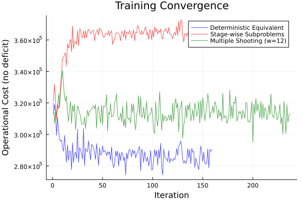


| Method | Mean Cost | Std | Violation % | Train Time |
|---|---|---|---|---|
| Deterministic Equivalent | 321189.0 | — | 48.66% | 158 steps |
| Stage-wise Subproblems | 364110.0 | — | 0.59% | 159 steps |
| Multiple Shooting | 319462.0 | — | 36.18% | 236 steps |