Star us on GitHub!
StarLearningToOptimize
Documentation for LearningToOptimize.
Learning to optimize (LearningToOptimize) package that provides basic functionalities to help fit proxy models for optimization.
Installation
] add LearningToOptimizeFlowchart Summary
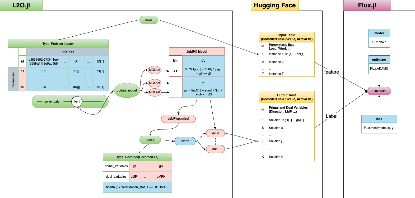
Generate Dataset
This package provides a basic way of generating a dataset of the solutions of an optimization problem by varying the values of the parameters in the problem and recording it.
The Problem Iterator
The user needs to first define a problem iterator:
# The problem to iterate over
model = Model(() -> POI.Optimizer(HiGHS.Optimizer()))
@variable(model, x)
p = @variable(model, p in MOI.Parameter(1.0)) # The parameter (defined using POI)
@constraint(model, cons, x + p >= 3)
@objective(model, Min, 2x)

# The parameter values
parameter_values = Dict(p => collect(1.0:10.0))

# The iterator
problem_iterator = ProblemIterator(parameter_values)
The parameter values of the problem iterator can be saved by simply:
save(problem_iterator, "input_file", CSVFile)Which creates the following CSV:
| id | p |
|---|---|
| 1 | 1.0 |
| 2 | 2.0 |
| 3 | 3.0 |
| 4 | 4.0 |
| 5 | 5.0 |
| 6 | 6.0 |
| 7 | 7.0 |
| 8 | 8.0 |
| 9 | 9.0 |
| 10 | 10.0 |
ps.: For illustration purpose, I have represented the id's here as integers, but in reality they are generated as UUIDs.
To load the parameter values back:
problem_iterator = load("input_file.csv", CSVFile)Samplers
Instead of defining parameter instances manually, one may sample parameter values using pre-defined samplers - e.g. scaled_distribution_sampler, box_sampler- or define their own sampler. Samplers are functions that take a vector of parameter of type MOI.Parameter and return a matrix of parameter values.
The easiest way to go from problem definition, sampling parameter values and saving them is to use the general_sampler function:
general_sampler(
    "examples/powermodels/data/6468_rte/6468_rte_SOCWRConicPowerModel_POI_load.mof.json";
    samplers = [
        (original_parameters) -> scaled_distribution_sampler(original_parameters, 10000),
        (original_parameters) -> line_sampler(original_parameters, 1.01:0.01:1.25),
        (original_parameters) -> box_sampler(original_parameters, 300),
    ],
)
This function is a general sampler that uses a set of samplers to sample the parameter space. It loads the underlying model from a passed file that works with JuMP's read_from_file (ps.: currently only tested with MathOptFormat), samples the parameters and saves the sampled parameters to save_file.
The Recorder
Then chose what values to record:
# CSV recorder to save the optimal primal and dual decision values
recorder = Recorder{CSVFile}("output_file.csv", primal_variables=[x], dual_variables=[cons])

# Finally solve all problems described by the iterator
solve_batch(problem_iterator, recorder)
Which creates the following CSV:
| id | x | dual_cons |
|---|---|---|
| 1 | 2.0 | 2.0 |
| 2 | 1.0 | 2.0 |
| 3 | -0.0 | 2.0 |
| 4 | -1.0 | 2.0 |
| 5 | -2.0 | 2.0 |
| 6 | -3.0 | 2.0 |
| 7 | -4.0 | 2.0 |
| 8 | -5.0 | 2.0 |
| 9 | -6.0 | 2.0 |
| 10 | -7.0 | 2.0 |
ps.: Ditto id's.
Similarly, there is also the option to save the database in arrow files:
recorder = Recorder{ArrowFile}("output_file.arrow", primal_variables=[x], dual_variables=[cons])Learning proxies
In order to train models to be able to forecast optimization solutions from parameter values, one option is to use the package Flux.jl:
using CSV, DataFrames, Flux

# read input and output data
input_data = CSV.read("input_file.csv", DataFrame)
output_data = CSV.read("output_file.csv", DataFrame)

# Separate input and output variables
output_variables = output_data[!, Not([:id, :status, :primal_status, :dual_status, :objective, :time])] # just predict solutions
input_features = innerjoin(input_data, output_data[!, [:id]]; on=:id)[!, Not(:id)] # just use success solves

# Define model
model = Chain(
    Dense(size(input_features, 2), 64, relu),
    Dense(64, 32, relu),
    Dense(32, size(output_variables, 2))
)

# Define loss function
loss(x, y) = Flux.mse(model(x), y)

# Convert the data to matrices
input_features = Matrix(input_features)'
output_variables = Matrix(output_variables)'

# Define the optimizer
optimizer = Flux.ADAM()

# Train the model
Flux.train!(loss, Flux.params(model), [(input_features, output_variables)], optimizer)

# Make predictions
predictions = model(input_features)
Another option is to use the package MLJ.jl:
using MLJ

# Define the model
model = MultitargetNeuralNetworkRegressor(;
    builder=FullyConnectedBuilder([64, 32]),
    rng=123,
    epochs=20,
    optimiser=Optimisers.Adam(),
)

# Train the model
mach = machine(model, input_features, output_variables)
fit!(mach; verbosity=2)

# Make predictions
predict(mach, input_features)
Evaluating the ML model
For ease of use, we built a general evaluator that can be used to evaluate the model. It will return a NamedTuple with the objective value and infeasibility of the predicted solution for each instance, and the overall inference time and allocated memory.
evaluation = general_evaluator(problem_iterator, mach)Coming Soon
Future features:
- ML objectives that penalize infeasible predictions;
- Warm-start from predicted solutions.